Confidence Intervals from first principles!

You would often hear Confidence Interval thrown around casually when your product metrics are too noisy and varying so much day over day that it looks nothing short of spooky wizardry. Well, stabilizing and understanding those metrics are a job for another day. For now, let’s delve deeper into what Confidence Interval (CI) really means and how you can apply it for your sprawling large scale Machine Learning application.

Imagine yourself in the middle of a lush green apple orchard, and like most worshippers of data, you wonder:

What would be the mean weight of an apple in this orchard?

A brute force solution would be to aggregate the weight of every single apple, and get its mean. Of course, this does not scale well as your population size (the number of apples) increases to several orders of magnitude greater than what your instrumentation can support. Is there a better way? Indeed there is. You could simply pick a few apples at random, and find their mean weight. We call this batch a sample, and the mean of this sample as the “estimate”, unlike the mean of the entire population of apples which was a “population parameter”.

But is this estimate the same as the true population parameter? The simplest way to verify this is to get another batch of apples, weigh them and duly report back. Alas, you would very likely observe that the mean weight is different this time.

Why did this happen? Every batch of apples you pick is going to be different, and consequently their sample estimates will differ too. This dissimilarity gives birth to what is called as a “sampling error” in estimates. It is the tendency of every sample to behave differently from each other. Note that, if all apples were similar to each other, this sampling error would be less.

In order to see how the different samples behave, you go and pick many samples of apples and obtain the mean weight for each one of them. If you have picked more than 30 samples with replacement (i.e once you computed the mean from a given sample, those apples were eligible for picking again), you will notice that the mean weight for all these samples lines up neatly along a bell curve for normal distribution. Is that a coincidence? No! The Central Limit Theorem (discussed in another article) provides us this guarantee.

In spite of knowing the mean weight for a bazillion samples of apples, our original question, what is the mean weight of an apple in this orchard’s population, still remains unanswered. ~As you would remember from the nursery rhymes where your parents should have taught you that the bulk of the normal distribution values lie around its mean (note that, this mean is different from the population mean we intend to find), and you can find out the range within which the mean is “likely” to occur.~ Is there a way for us to leverage the normal distribution of sample means to obtain the mean of the entire population?

We can, but not directly. Remember from your childhood conversations with your Data Scientist parents that the bulk of the normal distribution values lies around its mean. What did “bulk” mean? How much exactly is this “bulk”? Though we cannot answer this in absolute terms, by looking at the distribution curve we might be able to say that between value A and value B, C% of means lie.

Viola! I may not be able to provide the exact answer, but at least I can provide a range within which I expect the means (as the plural of mean, not as a means to an end) would lie. Since the sample mean is an “unbiased estimator” of the population mean [demonstrated in another article. For now take my word for it], we expect the population mean to follow the same distribution. Hence, we can extend our same line of reasoning to provide a range of values within which our population mean can lie with some chance.

Before we jump into hunting for the values of A, B and C, let’s discuss terminology. A and B are called the lower and upper Confidence Interval bounds, and C is called the level of confidence. C denotes how sure you are that the true population mean lies in the given range. It relies on the frequentist scientists’ belief of the world that probability of an event occurring in the future is the same as the frequency of its occurrence in the past. Note: this may not be a universally applicable assumption (for eg, in case of black swan events or in case of some cold start cache problems), but it is a good enough assumption for most use cases.

Now, let’s find out A, B and C. This is a relatively easier part to derive. We start with assuming some value of C (say, 95%, one of the most commonly used CI levels) and use that to compute A and B. Fortunately for us, many generations of statisticians (of course, all born after Newton and Leibniz) have used Integral Calculus to give us the area under the curve at different values of the random variable.

For our case, we are looking for the values such that area under the curve is 97.5%. Why not 95%? We would like to provide a CI symmetrical about its mean. Hence, to get a 95% CI, we will exclude the tail on both sides of the curve each weighing about 2.5%. Hence, we are looking for the area corresponding to z_p = 0.025 in a chart like below (taken from here):

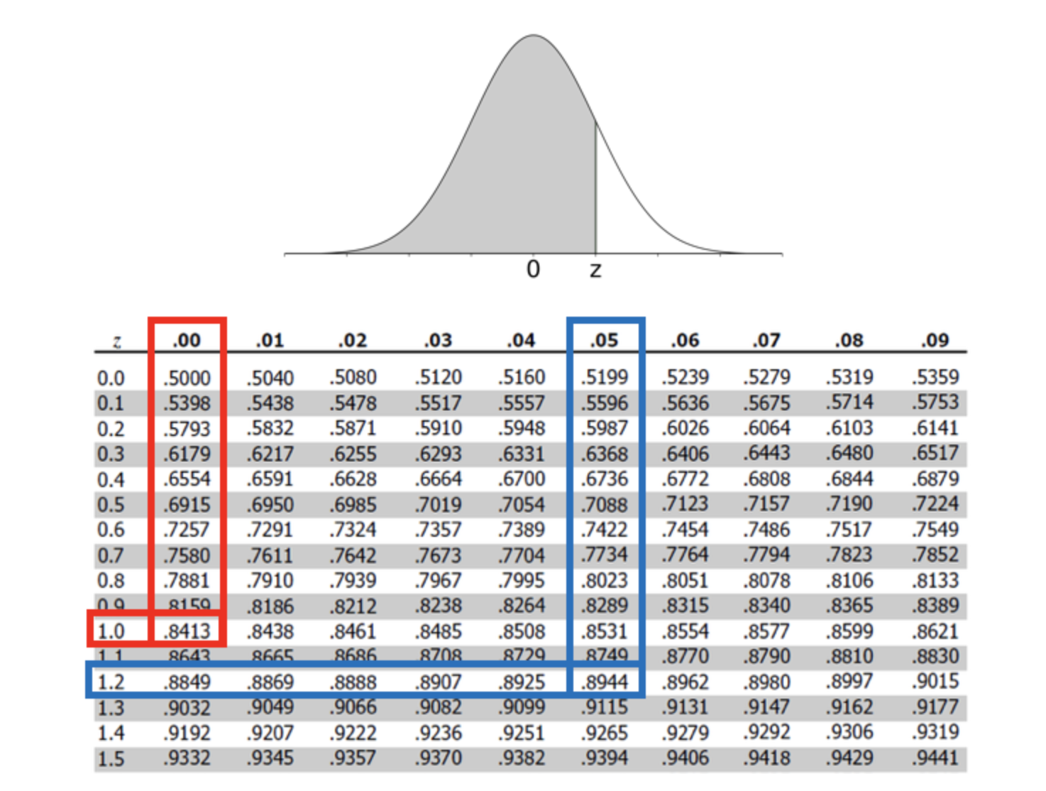Figure: The table entries for z is the area under the standard normal curve to the left of z

The value we gathered above is for standard normal distribution, i.e $\mu$ = 0 and $\sigma$ = 1. Since we never assumed our normal distribution to uphold these parameters, we need to scale the area obtained above by standard deviation.

Consolidating all of our hard work above, we obtain:

$CI=\mu{\pm}z_p*\frac{\sigma}{\sqrt{n}}$

If you have accepted the above formula without any qualms, you have yours truly to make an utter fool out of you, good sir! I quietly sneaked in a $\frac{\sigma}{\sqrt{n}}$ which should not have made its ways unexplained. This $\sigma$ here is the standard deviation of any random sample you have picked up (and likewise $\mu$ is the mean of any random sample). However, we use the $\frac{\sigma}{\sqrt{n}}$ and not $\sigma$ to scale up because $\frac{\sigma}{\sqrt{n}}$ is the unbiased estimator of standard deviation when the number of samples is large. Proving this would require another rigorous discussion, and so I am skipping here for the sake of brevity.

Now that we have derived the mathematical formulation of the CI, let’s now go back to our apple orchard. What would happen to the width of our CI if all the apples were almost identical? The different samples you would pick from such an apple orchard would tend to have similar average weight. And hence, the range within our population mean is expected to lie will become tighter. Mathematically, this translates to low variance, and a corresponding “less spread out” bell curve.

Consider again, the size of each sample. If I am taking a very tiny number of apples in each sample, my sample estimates for mean would fluctuate a lot. This happens because we have less information on which to base the interval, and hence the intervals will be wider. In larger samples, the effects by some unusual values is evened out by other values in the sample. Hence, larger samples will be more similar to each other. In the formula we derived for CI, this can be observed by increasing $n$ , the size of the sample.

Caution: If you are stuck in an orchard where you cannot take more than 30 samples, make sure to replace the $z_p$ in the above formula with a $t$ -distribution parameter. This is because for small samples (< 30), $t$ -distribution approximates the $Z$ -distribution.

Summary

We cannot compute the population parameter directly, and hence we need to estimate them. But this number will vary from sample to sample. This is what Confidence Interval tells us: if I were to take repeated samples, 95 % of the time the estimate for the population param would lie between A to B. That is, for every 100 samples we collect from data, 95 of them will have their mean in the given range and 5 will not.
Sample mean can be a point data, however population param is always expressed as CI
Sampling error: every sample would lead to different estimate for a population statistic. Hence the error between each sample is called sampling error.
Width of CI
- Variation within a sample: if the variance in samples is low, the CI will be tighter. And vice versa.
- Sample size: if we have less information on which to base the interval, the intervals will be wider. In larger samples, the effects by some unusual values is evened out by other values in the sample. Larger samples will be more similar to each other.
- CI Level the more confident we want to be (90%, 95%, 99%), the larger our CI will be. More level of confidence => wider interval for same sample size.
If the size of your sample is small (less than 30), use the t-distribution instead of z-distribution.